Part 7: Wavelet analysis and JPEG2000 compression
In the previous notebook, we introduced the Fourier Transform that represents images as harmonics or waves of varying frequencies. Using a local (block-wise) Cosine Transform, we were able to mimick the JPEG standard and compress images... at a significant cost: the introduction of blocking artifacts.
To alleviate this problem, engineers and mathematicians from the 80's came up with a new idea: the Wavelet Transform, that we are now going to present. But first, we need to re-import our standard libraries:
%matplotlib inline
import center_images             # Center our images
import matplotlib.pyplot as plt  # Display library
import numpy as np               # Numerical computations
from imageio import imread       # Load .png and .jpg images
And re-define our display routines:
def display(im):  # Define a new Python routine
    """
    Displays an image using the methods of the 'matplotlib' library.
    """
    plt.figure(figsize=(8,8))                     # Square blackboard
    plt.imshow( im, cmap="gray", vmin=0, vmax=1)  # Display 'im' using a gray colormap,
                                                  #         from 0 (black) to 1 (white)
def display_2(im_1, title_1, im_2, title_2):
    """
    Displays two images side by side; typically, an image and its Fourier transform.
    """
    plt.figure(figsize=(12,6))                    # Rectangular blackboard
    plt.subplot(1,2,1) ; plt.title(title_1)       # 1x2 waffle plot, 1st cell
    plt.imshow(im_1, cmap="gray")                 # Auto-equalization
    plt.subplot(1,2,2) ; plt.title(title_2)       # 1x2 waffle plot, 2nd cell
    plt.imshow(im_2, cmap="gray", vmin=-1,vmax=1)                 # Auto-equalization
Once again, we work on a simple axial slice:
I = imread("data/aortes/1.jpg", as_gray=True)  # Import as a grayscale array
I = I / 255                   # Normalize intensities in the [0,1] range
I = I[::2,::2]                # Subsample the image, for convenience
display(I)                    # Let's display our slice:

Wavelet transform
What if "Fourier" coefficients referred to well-located wavelets instead of pure, oscillating waves than span across the full domain? After all, when we write down music, we tend to use notes that have a well-defined frequency and duration... The Fast Wavelet Transform, introduced by Stéphane Mallat in 1989, is all about computing such a "music score" for images through the iteration of convolutions and subsamplings.
In the picture below, which is adapted from one of Mallat's papers, the input image is displayed on the right. At each layer, we compute highpass features through convolutions with oriented edge detectors, and a lowpass thumbnail that is subsampled before being fed to the same procedure once again. We stop when the "sub-sub-...-sub-sampled" residual is reduced to a single pixel, and the "Wavelet Transform" of the input image is then defined as the concatenation of all the feature maps, computed at different resolutions:
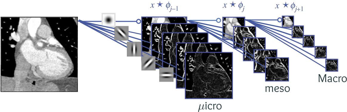
For image compression, we typically use three "highpass" filters at each scale, thus ending up with a nice set of thumbnails that fit into each other like Russian dolls:
# We use Gabriel Peyre's implementation of 2D wavelet transforms:
from nt_toolbox.general import *
from nt_toolbox.signal import *
from nt_toolbox.compute_wavelet_filter import *

def wavelet_transform(I, Jmin=1, h = compute_wavelet_filter("Daubechies",6)) :
    """
    2D-Wavelet decomposition, using Mallat's algorithm.
    By default, the convolution filters are those proposed by
    Ingrid Daubechies in her landmark 1988-1992 papers.
    """
    wI = perform_wavortho_transf(I, Jmin, + 1, h)
    return wI

def iwavelet_transform(wI, Jmin=1, h = compute_wavelet_filter("Daubechies",6)) :
    """
    Invert the Wavelet decomposition by rolling up the operations above.
    """
    I = perform_wavortho_transf(wI, Jmin, - 1, h)
    return I

wI = wavelet_transform(I)          # Compute the wavelet transform

plt.figure(figsize = (8,8))        # Square blackboard
plot_wavelet(wI, 1)                # Custom display routine, with a red tesselation
plt.title('Wavelet coefficients - with added recursive grid')
plt.show()

Multiscale pyramid. Here, the low frequencies sit in the upper-left corner and represent the image at coarser and coarser scales. To extract "bandpass" images as in the previous notebook, we simply have to zero specific bands in our Wavelet Transform wI:
def Wavelet_bandpass(wI, depthMin, depthMax) :
    wI_band = wI.copy()              # Create a copy of the Wavelet transform
    # Remove the low frequencies:
    wI_band[ :int(2**(depthMin-1)), :int(2**(depthMin-1))] = 0
    wI_band[ 2**depthMax:, :] = 0  # Remove the high frequencies
    wI_band[ :, 2**depthMax:] = 0  # Remove the high frequencies

    I_band = iwavelet_transform(wI_band)

    display_2( I_band, "Image",          # And display
               wI_band, "Wavelet Transform" )
If we just keep the coarser scales, we retrieve a "blurred" image:
Wavelet_bandpass(wI, 0, 4) # Scales 0, 1, 2, 3, 4

Wavelet decompositions produce features that are well-located:
Wavelet_bandpass(wI, 5, 6) # Scales 5 and 6

In sharp contrast to the Fourier bandpass images of the sixth notebook, these wavelet decompositions do not really suffer from ringing artifacts: oscillations remain close to the shapes' supports:
Wavelet_bandpass(wI, 7, 8) # Scales 7 and 8

Crucially, Wavelet Transforms perform very well in compression tasks at a cheap numerical cost. To illustrate this, we follow the same steps as in Part 6:
def Wavelet_threshold(wI, threshold) :     # Re-implement a thresholding routine
    wI_thresh = wI.copy()                  # Create a copy of the Wavelet transform
    wI_thresh[ abs(wI) < threshold ] = 0   # Remove all the small coefficients
    I_thresh = iwavelet_transform(wI_thresh)   # Invert the new transform...

    display_2( I_thresh, "Image",          # And display
               wI_thresh, "Wavelet Transform" )
    return I_thresh
Thresholding operations tend to preserve the sharpness of geometric features:
Wavelet_threshold(wI, .2) ;

If we compare our results to the 1:33 compressions of the previous notebook, the Wavelet Transform looks good!
Abs_values = np.sort( abs(wI.ravel()) )  # Sort the coefficients' magnitudes
print(Abs_values)                        # in ascending order...

cutoff = Abs_values[-2000]                # And select the 2000th largest value
JPEG2000 = Wavelet_threshold(wI, cutoff)  # as a cutoff
display(JPEG2000)


To remember: Multiscale image decompositions (pyramids), computed through a succession of convolutions and sub/supsamplings, have a long history.
Easy to compute (convolutions are cheap), these representations encode a multiscale prior: features at scale k should be computed locally as aggregations of finer descriptors at scale k+1.
From the 70's to the turn of the XXIst century, a great amount of effort was put into the engineering of convolution filters with optimal properties. The Daubechies filters or the CDF wavelets (used in the actual JPEG2000 standard) are prime examples of this research, which powers digital cinemas or MRI reconstruction softwares.
Convolutional "Neural Networks". But since 2012, the combination of GPUs and high-level automatic differentiation libraries (Theano, TensorFlow, PyTorch...) has changed the rules of the game: as we'll see on Saturday, filter weights can now be tuned automatically using gradient descent, and don't have to be hand-picked anymore.
This major breakthrough has allowed engineers to best fit their models to the available data, and to explore new families of convolutional architectures that were previously "too hard to tune" to be useful. This is impressive research.
But don't be fooled by the hand-waving, pseudo-biological intuitions that are often bundled with these methods. As should be clear by now, the "Neural Networks" in Convolutional Neural Networks is little more than a cool, but very misleading piece of mathematical jargon:
- Convolutional architectures are miles away from being "biologically inspired". They simply follow a well-known, wavelet-like algorithmic structure that encodes a multiscale prior on feature detection tasks.
- Models are "trained" using gradient descent; just like a ball that runs down a hill. No thought is ever modelled.
Final words. When marketing people put a biological neuron in their slides, they sell you a dream, not a product: "AI" simply doesn't exist. You should always be cautious (but optimistic) when reading about progress in the field:
- "Algorithms are opinions embedded in code", hypotheses that should be spelled out as explicitly as possible. The fine-tuning of parameters (with respect to a database) does not alter this fundamental rule.
- Hardware limitations put a hard cap on what we can deliver. So don't expect too much, too soon.